Ray Marching

The Theory

If tutorials are what you're looking for then I'd strongly recommend this video by SimonDev and this video by Sebastian Lague. I also came across this online book by Gabriel Gambetta. It's about graphics in general, not just ray marching, and I haven't taken a look at it yet but it seems very promising and I felt like sharing. Let me know if it's any good!

Ray marching is the process of finding a ray's distance to all objects in the scene and stepping the ray forward by the minimum of the distances found, so that the ray will never move inside of an object. If the minimum distance found is very small or zero, then we can say that a collision has occurred. Although it may sound expensive, many primitive objects as well as a number complex ones have well-defined distance estimation functions which can be calculated much faster than ray-triangle intersections. In particular, many fractals have relatively simple distance estimation functions. In addition, distance estimation is particularly good with rendering repeating patterns. It also makes soft shadows particularly easy, so I'll implement those as soon as they become available. The demo below shows the ray marching process for a single ray emanating from a green dot. Click and drag to change the ray's position and direction.

The green dots represent the positions visited by the ray as it travels, and the hollow black circles represent the distance estimations. The ray simply figures out exactly how far it can travel without intersecting anything and travels that far ahead. As you can see, the distance estimates get very small as the ray very nearly approaches an object. That's the secret to our soft shadows which I'll talk about down the line. The concept works equally well in three dimensions of course, although in that case it would be prudent to be much more careful about performance!

Shading

The first render will be of a simple sphere. I cast rays for each pixel, offset according to their positions, and test for collisions. If they collide, the pixel will be white, otherwise black. Of course this will amount to nothing more than the world's most inefficient circle-drawing algorithm, so I should add shadows in. For now, I'll use a method discussed down the line which just casts a ray from the light source to determine whether the point can see the light, and shade it accordingly.

What I eventually landed on was casting a ray from the light source towards the collision point. Once this ray collided, if it was too far from the collision point, we say that point is shadowed. You'll want to make this threshold much larger than the normal collision threshold, at least 10 times larger, or surfaces lit at a particularly shallow angle won't be shaded properly.

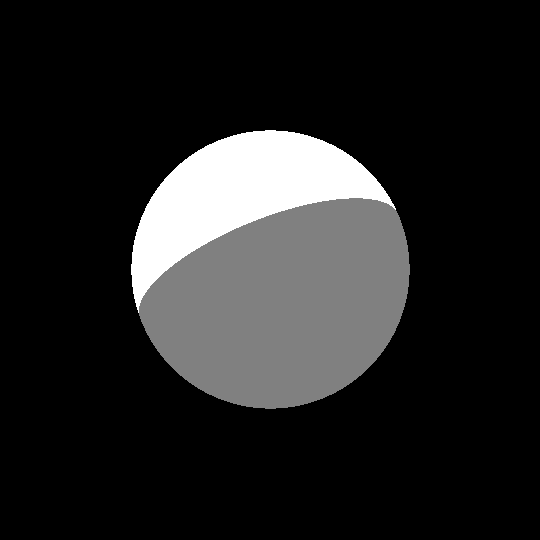
It's not too impressive yet, but it certainly demonstrates that the program is working. The next step is to properly implement lights. Lights can be fairly complex, they can be different brightnesses, colors, and as we'll see it pays to be able to set them as having different sizes as well. There are also different types of light, such as light sources that are so far away that all the incoming light is effectively parallel. For now, we'll stick with point lights and we'll make sure to set the falloff according to the inverse-square law. The below image is the same sphere lit by a red light and a blue light. It is also lit by a light at the camera's position to show the whole sphere.

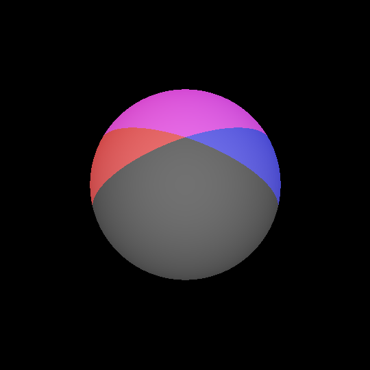
This picture really highlights an issue we have right now. Clearly, the self-shadows should be soft. Unfortunately, this has nothing to do with the relatively easy soft shadows between different objects. In this case, the change in brightness is related to the angle of incidence of light rays. In order to calculate that, we'll need the normal vector of the surface that was hit. There are a few ways of doing this, and one way that we probably shouldn't go with is defining normal functions for each of our objects, because for more exotic shapes it can be extremely difficult and involve a lot of math that I don't know. The method we'll be going with is to sample the distance field at a few points near the collision to get the approximate direction to the object being hit. To save time, we'll only sample the distance to the object that we hit, not to the entire scene.

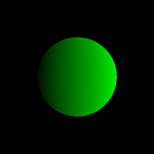
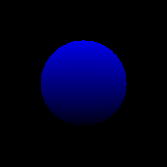
We can visualize the normals by interpreting them as colors. In the below image, each normal's x, y, and z value is mapped to the r, g, and b values of the pixels they correspond to.

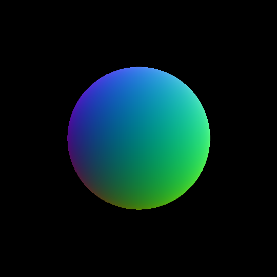
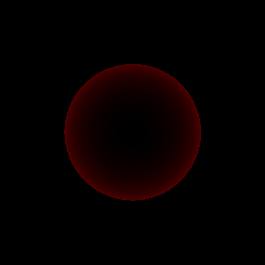
It's kind of difficult to tell, but this image is correct. It's easier to see if we isolate the individual channels:

Now that we have normal vectors, why can apply a reflection model. We'll use Phong reflection, which is a pretty standard choice, especially where realtime rendering is not necessary. This models the brightness of points on a surface as the sum of contributions from ambient light, diffuse reflection, and specular reflection. The ambient contribution is considered to come about by way of indirect lighting. The diffuse reflection models rough surfaces, and the specular reflections model an objects "shininess". Unfortunately, however, this model does not take into account the distance of the light source, so we'll have to figure that one out ourselves.

Have you ever wondered why objects twice as far away don't appear dimmer? After all, light obeys the inverse-square law, so objects twice as far away should appear a quarter as bright. Indeed, the amount of light hitting your eye from an object decreases by a quarter if your distance to it doubles, but its size also decreases by a quarter and these effects exactly cancel out. In reality, your eye measures the amount of light emitted by an object relative to its size in your peripheral vision. Or at least, that's what your brain measures. As a result, the distance between the viewer and the object being viewed doesn't matter when calculating its brightness, nor does the distance between the screen and the viewer, thank God. The distance from the object to the light, on the other hand, does.

The unit candela, abbreviated cd, measures the total output of a light source per solid angle, or steradian, abbreviated sr. Steradians are effectively a measure of the amount of your field of view that an object takes up. In essence, we want to measure the light source's brightness, reduce that according to the inverse square law, use Phong shading to calculate the amount that gets reflected towards the viewer, and then multiply that by some constant to get the actual pixel values. This last constant is what you're changing when you calibrate the brightness of a game by the way, it depends on the screen's brightness. And we'll just do that for each RGB channel independently. We'll say that a light source of brightness 1 will illuminate a unit square at a distance of 1 unit with a luminance of 1cd/m². So a unit square twice as far away would be lit at 1/4cd/m², and a square 3 times as far away would be lit with 1/9cd/m². A typical monitor has a brightness of about 350cd/m², so we'll take our final value, divide it by 350 and multiply it by 255 to get our pixel brightness.

We'll start with just the diffuse component of the lighting. This component is modeled as in Lambertian shading, where the brightness is the same regardless of the viewing direction and is proportional to the cosine of the angle between the vector from the collision to the light source and the surface normal - in other words, the dot product. We first calculate this value, then if it is non-negative, we will proceed to divide the light's brightness by the square of the distance between the collision and the light source and multiply it by our dot product value. We then multiply this by constants representing the color of the light and object to get the final values for each RGB channel.

Below is the program I used to generate this image. It's only the main code and excludes the actual library, in case you'd like to see the actual parameters for this scene. The full, final code is available through the GitHub link at the top of the page. This code will not work in the final version.

#include <stdio.h>
#include <stdint.h>

#include "utility/vec.hpp"

// Class definitions specific to this project.
#include "ray_march.hpp"

using namespace util;

int main() {
	int width = 1080/2;
	int height = 1080/2;
	
	float radius = 1;
	
	// Create the scene descriptor. Allocates space for one object, one parameter, and three lights.
	scene_descriptor sd(1, 1, 3);
	
	// Add a simple sphere to the scene descriptor.
	// "qid" -> "Quaternion Identity" -> "No rotation"
	sd.add_object_with_params(SPHERE, vecd3(0, 0, 0), qid, rgb(255, 255, 255), SPHERE_N, &radius);
	
	// Add lights to the scene.
	sd.add_light(vecd3(-0.5, -2, 5), 9600, rgb(255, 0, 0));
	sd.add_light(vecd3(-0.5, 2, 5), 9600, rgb(0, 0, 255));
	sd.add_light(vecd3(-4, 0, -2), 1000, rgb(255, 0, 255));
	
	// Create the camera.
	camera cam(vecd3(-4, 0, 0), qid, 1);
	
	// Create the image buffer
	uint8_t* img = new uint8_t[width*height*3];
	
	// Render the scene.
	cam.render(sd, width, height, img);
	
	// Save the image to file.
	char hdr[64];
	int hdr_len = sprintf(hdr, "P6 %d %d 255 ", width, height);
	
	FILE* fout = fopen("out.ppm", "wb");
	fwrite(hdr, 1, hdr_len, fout);
	fwrite(img, 1, width*height*3, fout);
	fclose(fout);
	
	delete[] img;
	
	printf("Goodbye!\n");
	
	return 0;
}
			

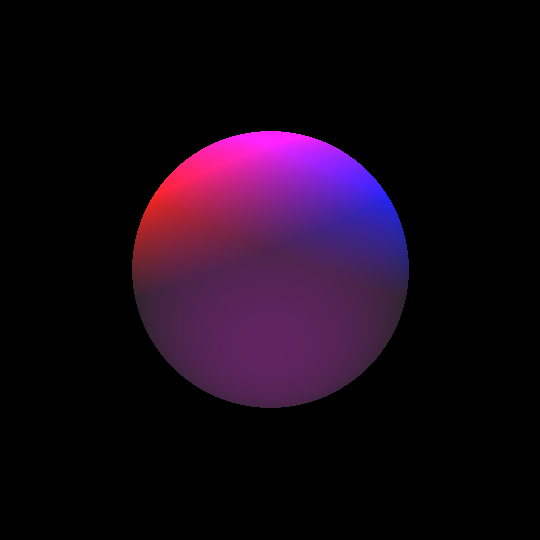
I'd say we have a pretty good render on our hands. We still have more to do, however. We need to include specular highlights in the image, in other words we need to be able to make it shiny. We should also include the ambient light, so that objects can appear to be lit indirectly. Ambient light is the easiest, it's just a constant brightness added to each point. For the test render the ambient brightness will be very high (40cd). You can see on the top of the sphere where the values get maxed out, we might want to decide to fudge the numbers a bit to prevent that later.

Next we'll do specular lighting. The objects and lights will have separate brightness and color for the specular and diffuse lighting, so that we can finely control the appearance of objects. The specular brightness is the dot product of R and V, where R is the direction a perfectly reflected ray would be traveling after bouncing off this surface and V is the vector from the point of collision to the viewer's eye. This dot product is close to 1 where perfectly reflected rays travel towards the viewer and closer to 0 otherwise. We then raise it to the power of a constant that defines the object's shininess. The higher the shininess, the faster this brightness approaches 0 as the reflected ray moves away from the viewer, causing the specular highlights to be smaller. We only use this calculation if both the dot product and the previous dot product we used for diffusion are non-negative.

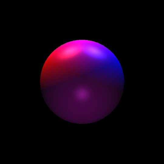
Now the sphere looks shiny! The specular brightness shown here is identical to the diffuse brightness, although it has a slightly whiter color. The highlight near the middle looks pretty good, but the other two seem quite a bit off. If you go in with a color picker, you'll see that this is because we're maxing out our color channels again. It's starting to look pretty bad, so lets start softening this out a bit. Our problem rests with this graph:

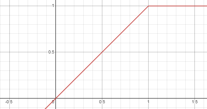
The x axis represents the brightness of the point and the y axis represents the brightness that we write to the pixel. Don't worry about the scales, they're arbitrary. The problem we're having is the sharp corner at the end there. The color gradient goes from smoothly changing to flat across a boundary line. It'd be better if we had a smooth change.

When trying to make a smooth function, its often better to think about the function's slope rather than its values at different points. We want a function with a slope of 1 at x = 0, and we want that slope to approach 0 rapidly as x approaches infinity. The best function for our purposes is the logistic function.

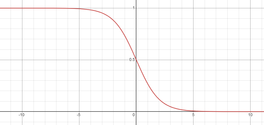
Honestly, this on its own could be modified into decent approximation, but instead what we'll do is modify it to match the slope of our desired function...

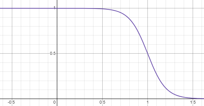
Then have Wolfram Alpha integrate it because I'll be fucked if I ever learn my integration rules...

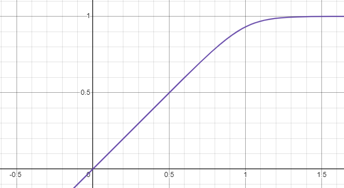
And voilà, we have our smooth color function! Hey, wait a second...

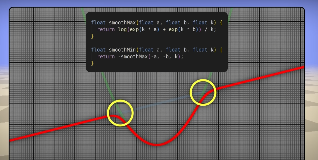
This function is exactly the same as the one for smoothing between distance estimators from that one video I linked at the start, albeit in a different form. Neat!

And now we have much nicer looking highlights. And, somehow, that just about wraps up the lighting model! Except of course for shadows, which according to some are very important.

Shadows

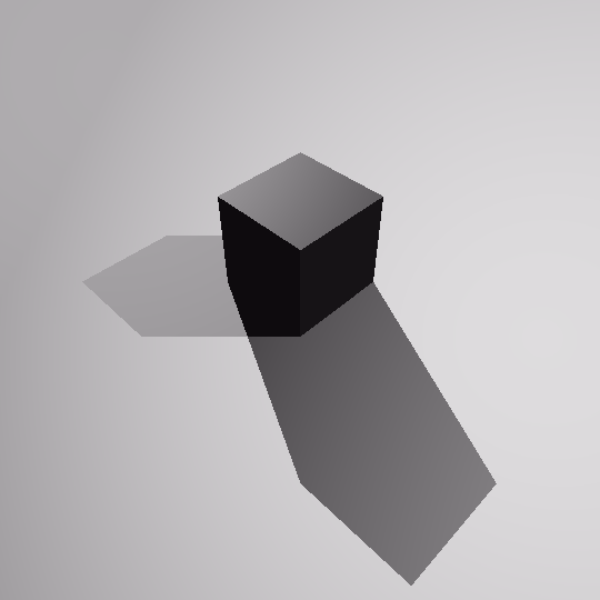
For these renders, we'll be using a cube sitting on a plane.

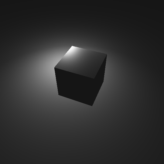
Very sad. Thankfully, there is a pretty straightforward way of calculating shadows. We can simply march a ray towards the collision point from each light source. If it hits the same location, we account for that light source. Otherwise, we skip it.

Now we just have to figure out soft shadows. Unfortunately, without casting more rays, the points currently in shade will always be in complete darkness. We can darken the points just outside the shaded area, however, by analyzing the behavior of the light ray. In particular, we want to know how close it came to hitting the cube. We'll record the smallest distance estimator value as the ray travels, and if it ever increases again then we'll say that this value is our closest approach. We'll also record the position the ray was in at that time.

Soft shadows occur because, in real life, points which have line of sight to an entire light source are lit fully, and points which have line of sight to none of the light are in complete shadow. The in between area of points which have line of sight to a portion of the light make up the soft edge of the shadow. In order to find this, we'll give the light a radius property and calculate its size from the perspective of the collision point, a value measured in radians. We'll then calculate the same value for the closest approach and use that to find the amount that the light is occluded.

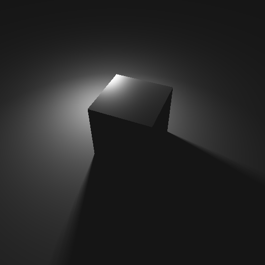
And here's another render I like. Can you tell what my favorite colors are yet?

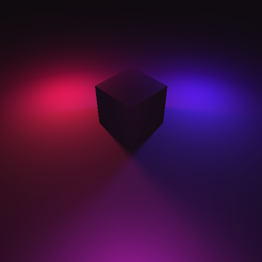
And we'll also add lights at infinite distance. These are lights that we model as being infinitely far away, which are good for light sources meant to imitate the sun. The direction to these lights is a constant everywhere in space and we don't apply the inverse square law for obvious reasons. These lights are also always sharp. Here's a render using a couple of those.

Rendering Fractals: The Mandelbulb

Once we finally have the lighting finished, we can try rendering fractals. We'll start by looking at the Mandelbulb, a 3D extension of the Mandelbrot set with a well-defined distance estimator. It's actually something of a posterboy for 3D fractal rendering.

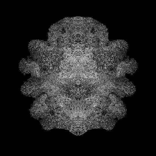
Unfortunately, this render is correct. The issue is that the surface is a fractal, and that the normal vector changes substantially over small changes in position. As a result, pixel values are radically different from pixel to pixel. In order to solve this issue, we have a few options. The most obvious is to just render way bigger images and then scale them down to reduce noise. I should get to work on that now because I'm going to be doing that in addition to every other improvement I make. The problem that this causes is that rending an image big enough will take way too long, so we'll need to finally do what I've been dreading and port it to the GPU.

It can take from 10-30 seconds to render an image of the Mandelbulb without rendering at high resolutions. At those numbers, even a brief, low quality animation is out of the question. Thankfully, the GPU code is so similar that I should be able to use preprocessor directives to inject GPU-specific code into the source when a macro is defined. At the heart of my code, the difference is that the GPU code uses a kernel and the CPU code uses a pair of nested for loops. Both of them utilize the same structure and both support the same pointer-to-distance-function/shader-function magic. The code should continue to work both on the GPU and the CPU.

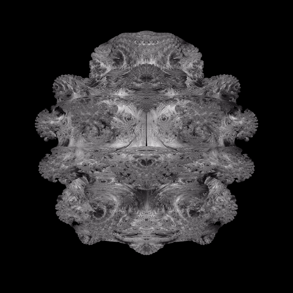
The below image was rendered at 16384x16384 pixels and scaled down to 1024x1024. Click it to see the 4096x4096 version. The full image took a few minutes to render out on an RTX 3060, please keep in mind that this is all before optimization.

One way we can significantly speed up the render is through an adjustment to the algorithm. I found the paper proposing the idea on a blog by Adam Celarek, although the paper itself contains no attribution. You can find the paper on his blog here or on my site here. The gist of it is that very nearby rays often fall inside each other's distance estimation radii, so redundant calculations can be reduced by only calculating the distance estimations for some of the rays until they diverge. This algorithm can actually, feasibly improve performance on any render. In particular it improves performance for high resolution renders of highly concave objects, like fractals!

In my implementation, I'll have each GPU thread compute the primary ray and keep track of its associated secondary rays. It will calculate the point at which the secondary rays diverge and launch them as their own rays at that point. Here's a render only including the contributions from the primary rays, the pixels controlled by secondary rays are left black.

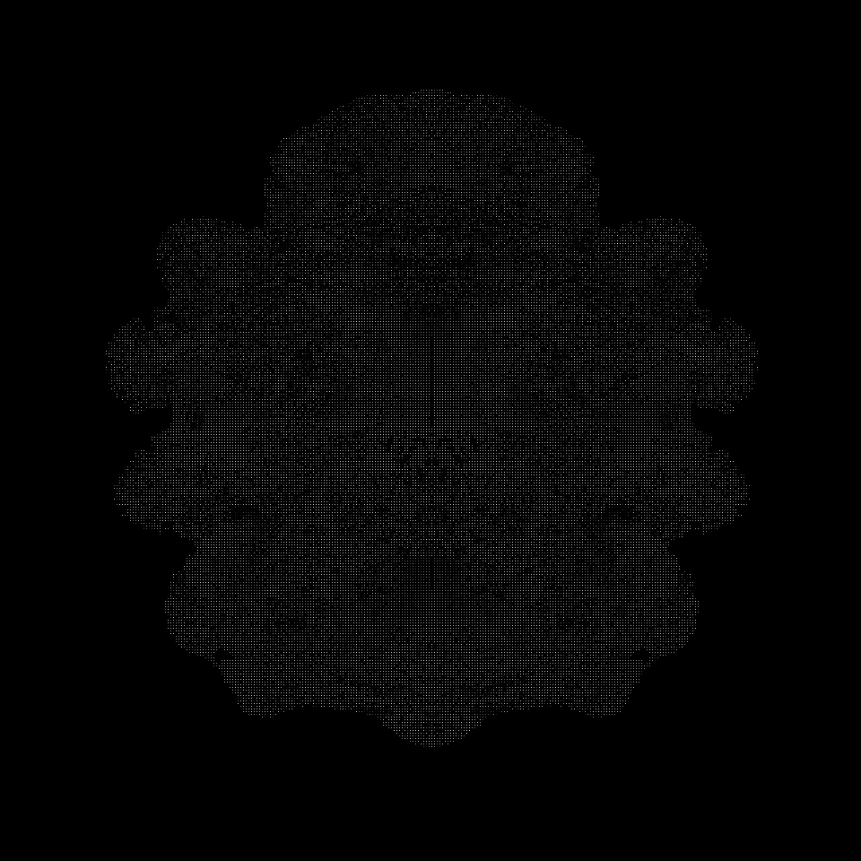
Funny looking! You'll want to zoom in on that to actually see what's going on. Only 1/9th of the pixels have been written to. The crux of this algorithm is in finding the minimum height of the intersecting circles generated by the last two distance estimations. And we do this at every step of the ray marching process. This value is represented by the dashed black line in the graph below.

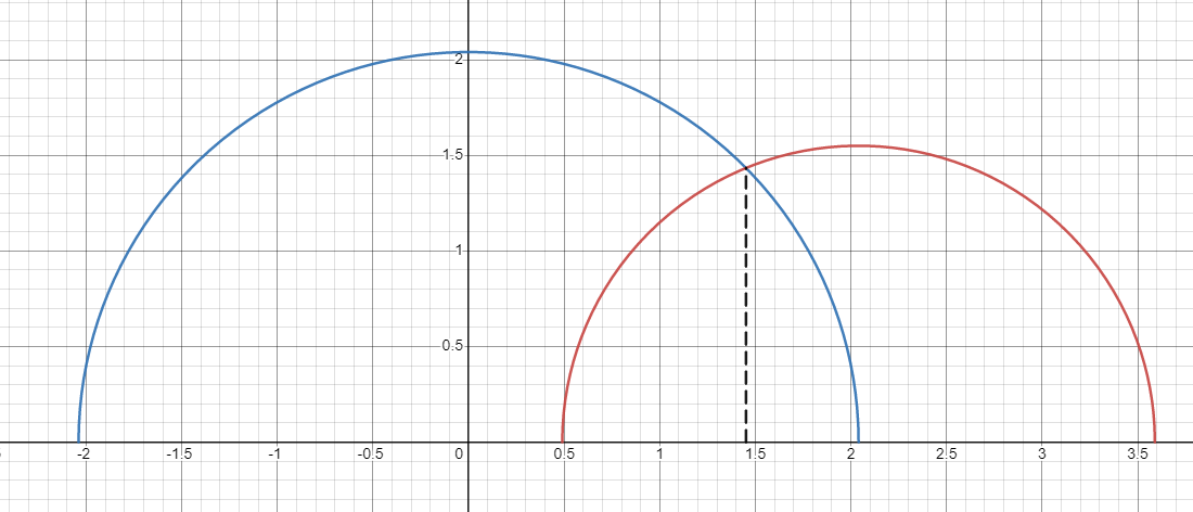
Investigating, you'll find the equation for that value is r₁ · sin(cos^-1(1 - r₂² / (2r₁²))) where r₁ and r₂ are the radii of the first and second circle. If you chose to investigate the trig functions, you'll find that the equation can actually be reduced further to r₁ · sqrt(1 - (1 - r₂² / (2r₁²))²). It can of course be reduced further, although its current form is probably about the fastest for our purposes. Once the distance of the farthest secondary ray exceeds this value, all secondary rays get launched as their own independent rays. A CPU implementation could leverage the fast conditional logic of the CPU to implement this algorithm via a branching tree structure for additional speedup, although it would still be much slower than the GPU.

Three images were rendered. They were rendered using 2, 1, and 0 layers of secondary rays (24, 8, and 0 secondary ray(s) per primary ray, respectively). The last one effectively imitates the old way of rendering, although with slight additional overhead because the logic for performing the secondary raycasts is still present. They took 64.36, 61.27, and 56.24 seconds, respectively. All renders were done at 6240x6240. Pretty unfortunate. That's because I made a vital mistake. In my implementation, each thread was responsible for not only the primary rays associated with the pixel it was rendering, but the secondary rays as well. Really, we should write two kernels. The first builds an acceleration structure by casting the primary rays and the second casts the secondary rays using the acceleration structure.

Wow, was that awful to implement. The scene descriptor passed to the first kernel, which has pointers to objects with pointers to distance estimation/shading functions, was being destructed at the end of the function call. This destructed the objects pointed to by the class (on the GPU and the CPU), causing it to crash when the second kernel attempted to call the functions on those objects. The solution was to pass the scene descriptor by reference, which is a whole other thing because you have to fill out this data structure on the CPU and then copy it to the GPU so that the value pointed to by the reference is accessible on the device. You can't just declare the variable as living on the device and then write to it like you can for arrays, because it isn't managed memory, and you can't initialize it on the device anyway because when you initialize the class it tries to call the constructor, which isn't supported for device variables.

Anyway, the time to compute the image with 8 secondary rays per primary ray went down to 44.33 seconds, and with 24 secondary rays it was 46.92 seconds. A healthy 21% performance increase. The image produced by that last render, scaled down to 2048x2048, is included below.

Wait... What is that?

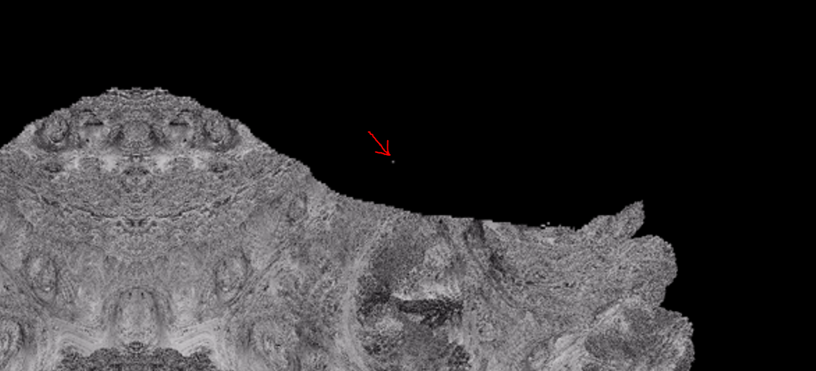
Huh. I wonder what it looks like in the original render.

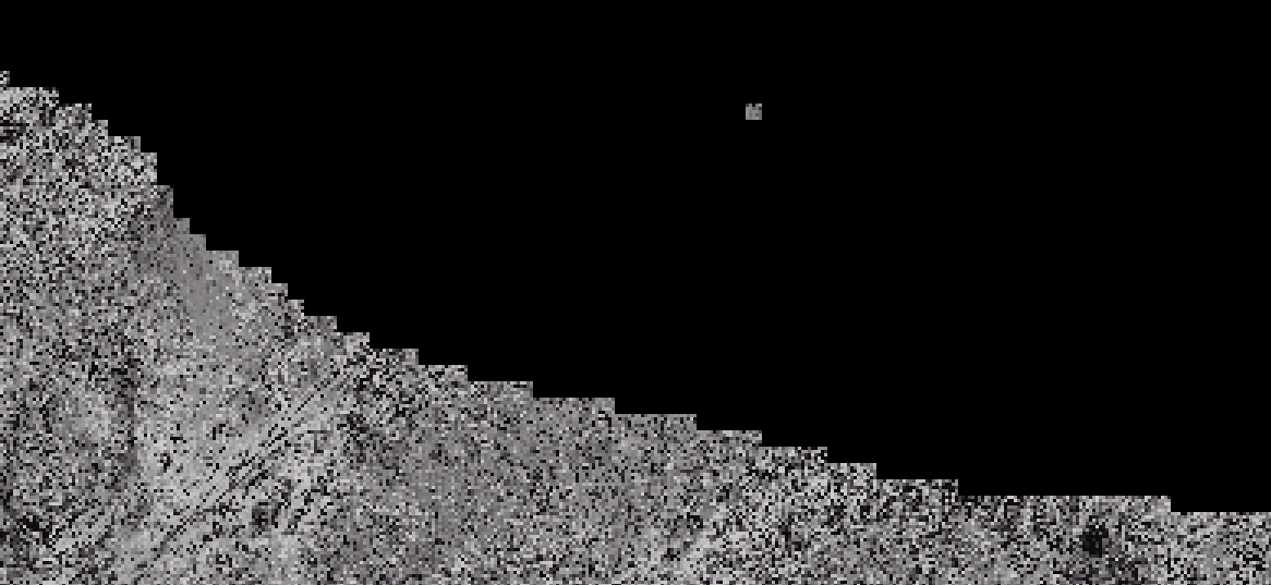
I can't believe I chose this over sanity. This was being caused because the z component of the secondary rays were the the reverse of the z component for their primary rays - go figure. Here's the render, for real this time, and I also went ahead and rendered it at 18720x18720. The full image took 6 minutes and 20 seconds to render.

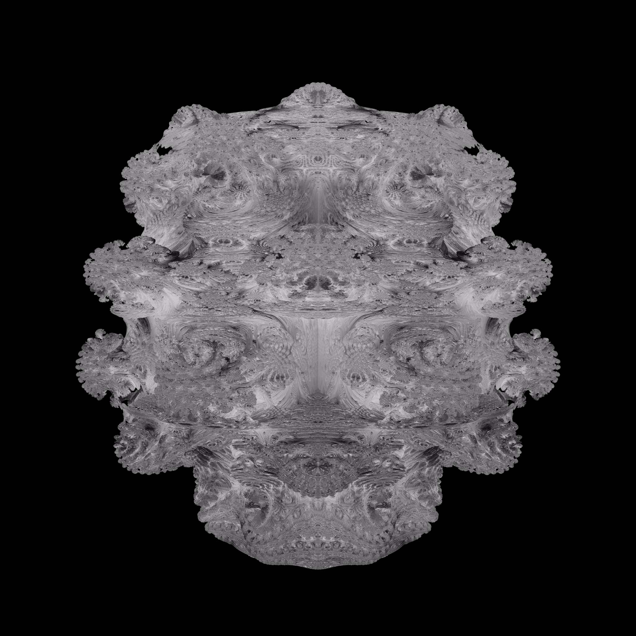
By the way, you might notice that these renders are upside down. Don't worry about it.

The next thing we'll want to try is applying different shading functions to different objects. That way, we can create a different shader for fractals and maybe we can do some fancier tricks later, but probably not. I'll save that for the raytracer. There are plenty of interesting shading functions for the Mandelbulb but the first step is to throw out the specular reflections and model the Mandelbulb as purely Lambertian diffusion, which is just the diffuse term in our Phong reflection model. We'll also keep the shadows and ambient lighting. The next step is to implement ambient occlusion to give better lighting hints when shading the fractal. The paper references another presented at SIGGRAPH 2006 which neither I nor the author of the other paper seem to be able to understand properly. The paper I linked uses a different and very straightforward method which my model, being based around pre-rendering images rather than realtime rendering, won't be able to use.

I will be sampling the distance function along the normal vector of the collision point. If the points along the normal have low distances, then the collision point is likely within a cavity and should be occluded. In essence, I will be sending a ray along the normal of the collision point and stopping it after only a few steps. The further it travels, the less the point is occluded. In particular, what we want to know is the ratio of the distance traveled to the initial distance estimate. For a completely unoccluded point, the distance estimate should double every time. Once the ray has a distance estimate that is smaller than the previous one, or the step limit is reached, we divide the ratio of the second-to-last estimation (the one that was bigger than the very last estimation) to the first estimation. This ratio should be 2ⁿ for an unoccluded point, where n is the number of steps taken, and its log₂ should be n. Therefore, the occlusion will be the log₂ of the ratio we took, divided by n. We use the log because otherwise the ambient occlusion would quickly approach 1 (representing no occlusion) for some pretty small cavities. We'll also make sure to cap the occlusion at 1 because we're working in approximations, and although it should never exceed that value in theory, it is very likely that it will in practice. This method also doesn't really work for objects with sharp corners, by the way.

The next addition is a glow effect. This one is pretty simple: We just have the secondary rays record their closest approach and, if they miss, we color them based on how close they got to the fractal. Later, I'll probably add actual code so the glow can be specified per-object and so forth. However, it is 4 in the morning and I just want to get this render kicked off so I can go to sleep and wake up to a nice video. The last one is just coloring the fractal, which we can do based on the collision point's distance from the origin. All of that combined produces the render below.

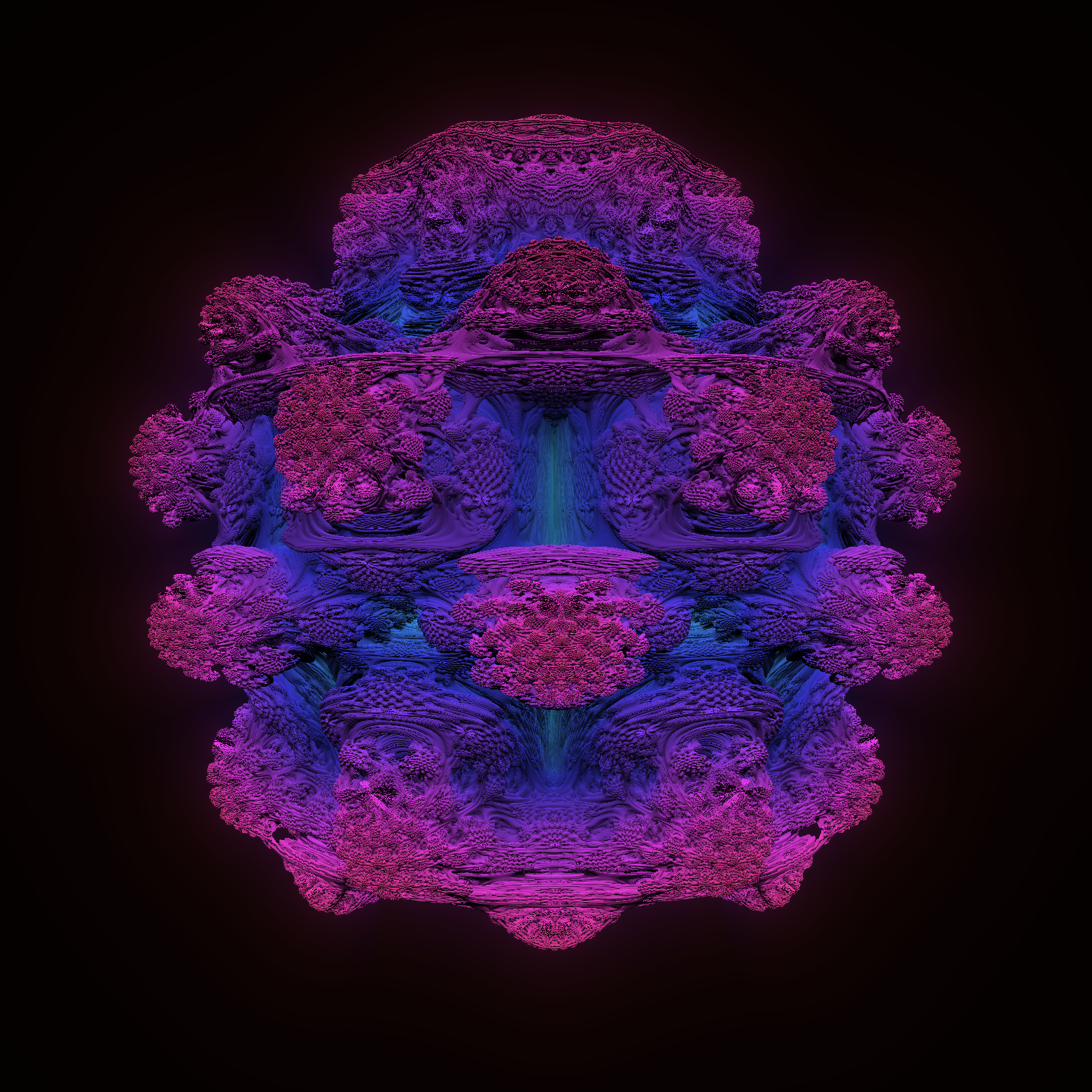
That all combined makes for a substantial upgrade! Now all that's left to do is animate it. I took a lot of care in making the animation. The Mandelbulb changes shape in a smooth fashion, and the camera moves as the Mandelbulb changes size. I rendered at a high resolution and what I felt was enough frames, and I tuned the parameters to get everything the way I wanted it to look. The parameters for the animation are the same as the image above, I rendered them out back-to-back. By the way, don't forget to wrap your cudaFree() calls in error checks... otherwise you might have a memory leak without realizing it and cause the program to crash an eighth of the way through your overnight render. Just a tip. Also, this video loops perfectly.

What Now?

There is so, so much I never got to in this project. With ray marching, you can combine objects in interesting ways! Like by smoothly blending them or taking their intersections, you could build a whole tree of objects that have unique shading and distance functions, and which interact in complex ways, you can take the space and make an object or multiple objects repeat forever in every direction. You can make an infinite series of objects within themselves, and you can make countless interesting fractals, many which don't resemble the Mandelbulb at all. One day, I will be returning to this engine. For now, I'm focusing on new projects.