Newton's Fractal
Newton's Fractal is a fractal produced by iterating Newton's method for approximating the roots of a function. Notably, Newton never new about the existence of this fractal, and could scarcely have known what it loked like without the modern technology of our time. I'll be going over the basics here, but 3Blue1Brown has a much better explanation here that I'm going off of and also stole the color scheme from.
Newton's Method
Newton's method for approximating the roots of a function should ring a bell for anyone who has taken a calculus course. What we want is to find the x values where some function f(x) equals zero, an extremely common question to ask in many disciplines and in particular in graphics (both 2D and 3D). We do this by finding where the tangent line of f(x) at x intersects the x-axis, and that becomes our next guess. We do this by taking the derivativew of f(x) to get the slope. Our next guess can then be written as:
pn+1 = pn - f(pn) / f'(pn)
We can then apply this function repeatedly until we get an approximation with a sufficient degree of accuracy. This usually only takes a dozen or so steps for sufficient accuracy, but for most quintic formulas there are numerous guesses you could make that take much longer to approach a root and whose behavior is very unpredictable. We map these values by taking each pixel, converting its position to a complex number, iterating it a dozen times with Newton's method, and coloring the original pixel based on which root its point approached.
Creating a Basic Render
I wrote up a quintic class that stores a quintic equation's coefficients as real numbers. It's constructor also takes the derivative of the polynomial which is trivially easy when we're working with polynomials only. I also put together a very simple rgb class for storing the colors and a complex class for simplifying the code when working with complex numbers. I could have imported my utility library which includes a complex class, but that seemed like overkill. I then used these classes to produce the basic render based on the above description of the algorithm. This image was rendered at 3840x2160 and scaled down to 1920x1080.
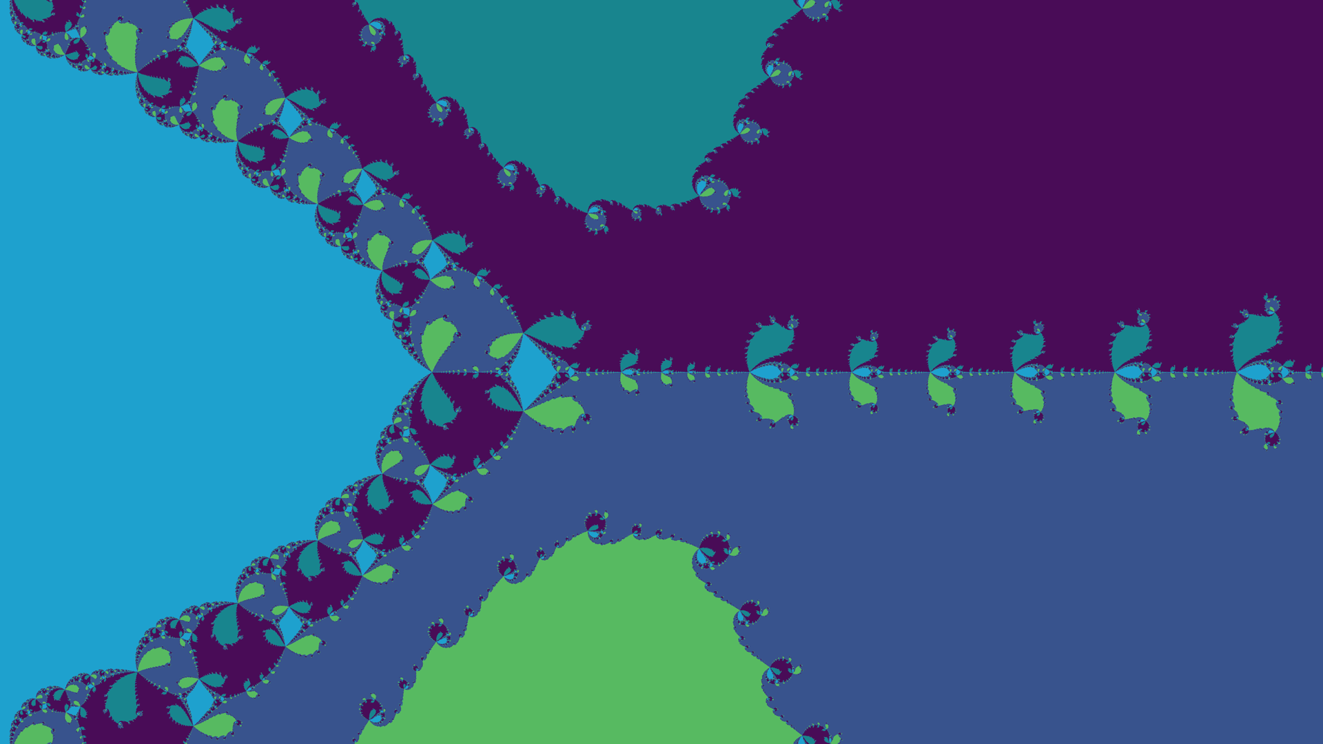
As you can see, there are 5 colors which generally correspond to 5 distinct regions of the plane. These are the regions where points relatively quickly approach one of the function's roots. The borders, however are chaotic. You can think of the points in this region as not knowing where to go, they tend to follow an unpredictable path to one of the roots. Sometimes, they get trapped in an attracting cycle and never approach a root, although this is very rare and doesn't ever occur for the quintic used in the above render.
Animating the Roots
For the above render, I used a calculator to find the roots of the quintic equation. There is no way to determine the roots of a quintic for certain using an equation, you can only approximate them. However, there's a trick we can use to provide better functionality. Instead of defining the polynomial and its roots separately, we can define the roots and calculate the polynomial that corresponds to them. This is relatively straightforward, we just take the roots and use them to write the function out in root form, like so (where r1 through r5 are the roots):
f(x) = (x - r1)(x - r2)(x - r3)(x - r4)(x - r5)
Deriving this isn't so easy, unfortunately, so we'll have to multiply it out in order to produce the final polynomial. That gives us this lovely little equation:
f(x) = x5 - (r1 + r2 + r3 + r4 + r5) · x4 + (r1r2 + r1r3 + r1r4 + r1r5 + r2r3 + r2r4 + r2r5 + r3r4 + r3r5 + r4r5) · x3 - (r1r2r3 + r1r2r4 + r1r2r5 + r1r3r4 + r1r3r5 + r1r4r5 + r2r3r4 + r2r3r5 + r2r4r5 + r3r4r5) · x2 + (r1r2r3r4 + r1r2r3r5 + r1r2r4r5 + r1r3r4r5 + r2r3r4r5) · x - r1r2r3r4r5
Which, believe it or not, is much easier to derive. Especially because the roots are all known, so this can be simplified to a normal-looking polynomial by evaluating the huge expressions including only these values. Plus, we don't have to actually write these out in the code. We can just use nested for loops to generate the sequences that we need for us. No concern for performance here, we need to evaluate that equation only once per frame.
I will say that I got hung up on the idea of generating the polynomial from the roots. Consider for example the following trinomial:
f(x) = (x - 2)(x + 2)(x - 1)
This equation expands to the following, and produces the graph given below:
f(x) = x3 - x2 - 4x + 4
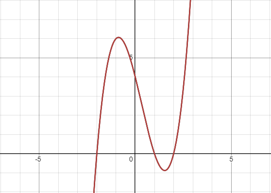
It is easy to see, given either the graph or the first form of the equation, that f(x) has roots of 2, 1, and -2. Another thing that's clear is that it must have exactly three roots. After all, this function (in the first form provided) is zero if any of the three multiplicands is zero. And if none of them are zero, then the function cannot be zero. There is no triplet of non-zero numbers whose product is zero, and this holds true for complex numbers. If you look at some other trinomials, you'll also see something else, they always have at least one root. It's clear that they must always have at least one root, because they approach negative infinity as x decreases, and positive infinity as x increase, so they must cross the x-axis somewhere.
So, we know (or we think we know, at least) that all trinomials must have a real root, and that it must have no roots other than those we specify. So what happens if you don't specify any real roots, only complex ones? It turns out to be fairly simple: It produces a polynomial with at least one complex coefficient. As it happens, our first idea (that trinomials always have a real root) only holds true for polynomials with real coefficients. And all of this generalizes to any polynomial of odd order (Polynomials of even order don't need to have a real root, even if they only have real coefficients).
I like to think of it like this: If our polynomial has complex coefficients, then the output can be complex even when evaluating it for real numbers. If it only has real coefficients, and therefore the output can only be real assuming the input is real, then for the output to go from negative infinity to positive infinity, it must cross the x-axis somewhere. However, if the output can be complex, this is no longer true. You can easily go from any point on a plane to any other without crossing the origin. In fact, as we move the function's input from negative infinity to positive infinity, it's theoretically possible for the function's output to touch every point on the plane except zero. Keep in mind that I've been talking strictly about differentiable functions.
I quickly swapped out some of the code so that quintics now store their coefficients as complex numbers and added a constructor so that a complex number can be initialized from a real, and it outputs the same image as before. I coded up the constructor that takes a set of roots and produces the necessary quintic.
Rendering with Different Roots
When I plugged in the roots to x5 + x2 - x + 1, it produced that exact equation, which I was not expecting! This is because there are an infinite number of quintics with those roots. Presumably, however, 3Blue1Brown (who I copied the quintic from) was using the same technique to find quintics with arbitrary roots. Indeed, when I moved one of the roots to another position which 3Blue1Brown had used, I was able to produce an identical image - within a small margin for error, given below.
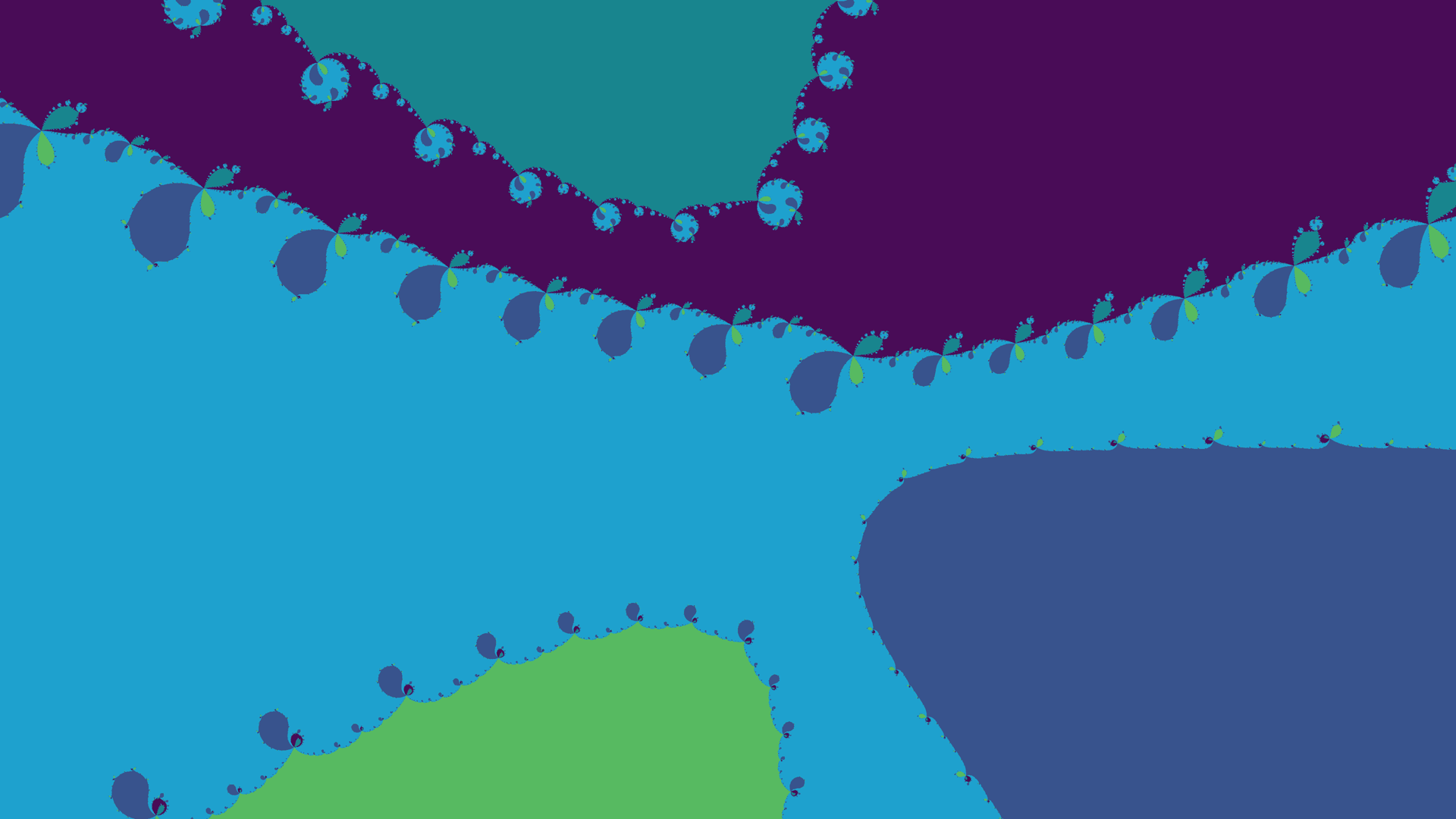
Of course, the next step I took was to render an animation with one of the roots changing. The below looping video has the real root alternating from -1.325 to 0.675 according to a sine wave.
Speeding Things up a Little
Unfortunately these renders are already taking hours. That means it's time for my favorite trick: GPU acceleration. I will be retaining the CPU functionality, however. I also want CPU code using these libraries to look identical to GPU code. The only difference should be a preprocessor directive to compile for GPU. The first step is to pull out the iteration function from main.cpp and into the library.
I'll create a camera class that holds the values used for converting between complex space and screen space. A camera object will provide a render function that we pass the roots to. Member functions cannot be GPU kernels, so this will be a standalone function that you pass the camera to. I also pulled out the code that allocates and deallocates the buffer to hold the image, and the code that saves the image to a file to remove any memory management that would otherwise be necessary on the user's side. This is especially important because the allocation and deallocation are performed differently depending on whether you're using the GPU. Finally, I created a render function that either calls the real render function or launches the render kernel depending on whether the code is using the GPU. Now, the render function looks like a member function even though it's just a proxy to the code that actually does the rendering.
Now, the code in main.cpp looks like this:
#include
#include
#include

#include "camera.hpp"
#include "quintic.hpp"

int main() {
	printf("Hello Quintics!\n");

	// Render parameters
	const size_t width = 1920;
	const size_t height = 1080;

	const size_t iters = 16;

	const size_t frames = 192;

	camera cam(width, height, 0, 0, (float) 16 / 3, (float) 9 / 3); // 16:9

	// Colors for each root.
	rgb colors[5] = {rgb(30, 161, 206), rgb(56, 83, 141), rgb(73, 12, 87), rgb(87, 186, 97), rgb(24, 133, 142)};

	// Allocate space for the output files' names and headers.
	char fn[64];
	char hdr[64];

	for (int f = 0; f < frames; f++) {
		printf("Frame %d...\n", f);

		float t = (float) f / frames * 2 * 3.14159;

		// Define the roots
		complex roots[5] = {complex(sin(t) - 0.325, 0), complex(0.662, 0.562), complex(0.662, -0.562), complex(0, 1), complex(0, -1)};

		// Render
		cam.render(roots, colors, iters);

		// Save to file.
		sprintf(fn, "./out/%03d.ppm", f);
		cam.save(fn);
	}

	return 0;
}
Now that I've prepared the library, I can begin adding the GPU code. The first step is to add the __device__ and __host__ qualifiers to most of the functions. This will tell NVCC (Cuda compiler) to compile these functions for execution on the GPU as well as the CPU. The real render function will get the __global__ qualifier, however, which will tell NVCC that this function is a kernel that can be called from the CPU. The __device__ functions can only be called from the GPU.
But wait! There's one more thing we have to do and it is extremely important. We must pass the camera by reference. Otherwise it will be destructed when the render function returns, and the image data will be freed. When we try to save that data to an image, the program will crash. This is a bit trickier than usual, however, because in order to pass an object by reference we'll need to ensure that the object is accessible from the GPU. To solve this issue, we have the proxy render function allocate space for a camera on the GPU and copy it over, then we pass that object by reference to the kernel. Don't make the mistake of passing an object with allocated memory by value to a kernel (or to any function, but especially to a kernel because you absolutely will not want to be having a copy constructor called for every kernel call).
We also need to copy the roots and colors to the GPU because they're being passed by pointer. Once that's finished up, the GPU code is complete, and it was one of the largest speedups I've obtained so far in a project. The video, which previously took nearly an hour, now takes only seconds.
There was an idea I had to scale the quintic to produce other functions with the same roots, that would produce different fractals. While you certainly can scale them, the resulting images are identical. After a bit of thinking, I realized that this is because we're scaling both the function and its derivative by the same amount. The step size in Newton's method is calculated as f(p) / f'(p). When we scale the qunitic by 5, we're changing the step size calculation to 5f(p) / 5f'(p), which of course doesn't change it at all. It seems to me that there can only be one quintic with a given set of roots, not accounting for a scaling factor. If so, then the Newton's fractal must always be the same for any given set of input roots. The only way to change it would be to use a higher-order polynomial which has some roots overlapping. So, there's that.
Animating Render Quality
One thing you can modify about the render that changes it quite substantially is the number of iterations of Newton's method that you perform. If you use zero iterations, each point just gets colored based on how far it is from the nearest root, producing a Voronoi diagram. With each additional step, the fractal becomes more sophisticated and closer to the true fractal. Below are renders at 0 through 5 iterations:


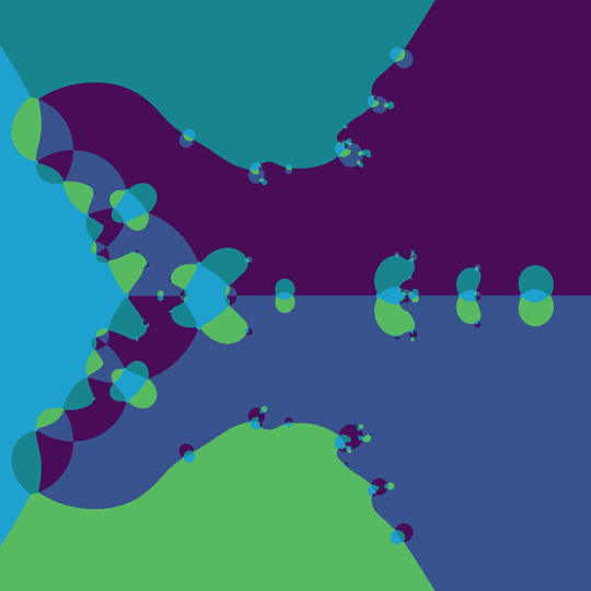
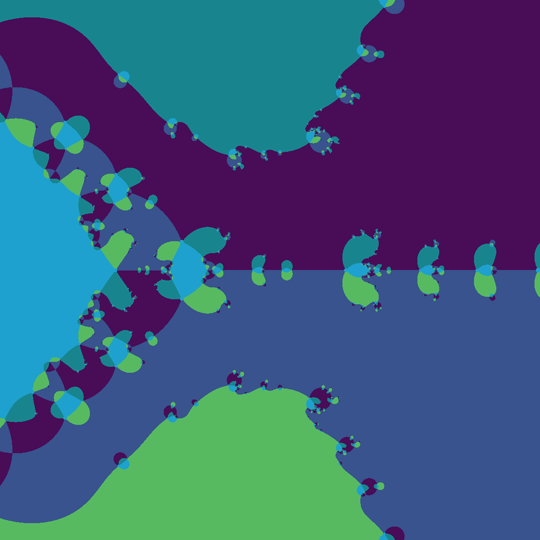
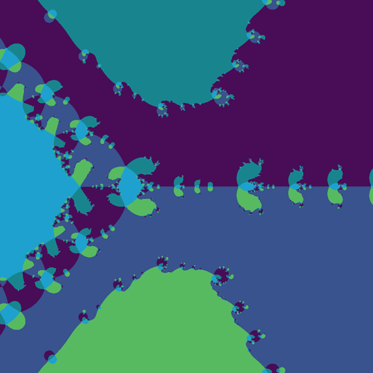
Clearly, the number of iterations is a discrete property. If we could somehow renormalize it, we could produce a smooth animation of the iteration count increasing. I have a theory that I can record the positions visited by each point after each iteration and then interpret the sequence of points as a Bezier curve. We can then follow the point as it moves through the curve and produce an animation, effectively, of the iteration count slowly increasing.
In order to implement this, I'm going to change the render function so that it no longer produces an image but rather records the positions visited by each point into a structure. This structure should not need to be bigger than a gigabyte or two even for very high quality renders. Unfortunately, performing the Bezier interpolation requires copying this data. As a result, we run up against memory restrictions relatively quickly. I'd recommend using the CPU version for this render, it's a good bit slower but won't fail from memory restrictions. The below video was, however, created with the GPU version. We see the fractal develop from 0 iterations up to 15.
Additional Renders
Below I've included some renders I created using this program. The first is a straightforward zoom on -0.314.
This next one can be a bit nauseating if you look at it for a long time, to be honest... But I love it regardless! It looks like the camera is zooming in and out, but that is an illusion. Scaling the roots away from the origin is identical to zooming the camera in, and the opposite is the same as zooming the camera out. At least I'm pretty sure it is. So, when the sum of the roots' velocities is away from the origin, I guess our brains perceive that as the camera zooming in, and when the roots tend inward, it looks like the camera is zooming out. In reality, the camera is fixed in place.
I made this one by generating a Bezier curve for each root to follow, so they all just meander around aimlessly. I ensured that the curves and their derivatives both end and start on the same value, so that the video loops nicely.