The Bifurcated Mandelbrot
The Math
The bifurcated Mandelbrot demonstrates the relationship between the Mandelbrot set and the logistic map bifurcation diagram, two seemingly unrelated aspects of chaos theory. It begins with the logistic map. This iterative equation is defined as xn+1 = r · xn(1 - xn) and was popularized by biologist Robert May as a method of predicting the change in populations of species in an environment with limited food. It quickly became a staple of chaos theory due to its unique behavior, predicting that some populations never stabilize but rather that they fall into complex repeating patterns. The simplest of these would be a population that increases on even years and decreases on odd years, but some fall into complex cycles of rising and falling. For example, the below graph represents the population size over the course of 30 generations with an initial size of 0.5 and a constant r of 3.7. Note that the y axis is the ratio of population to the carrying capacity of the environment.
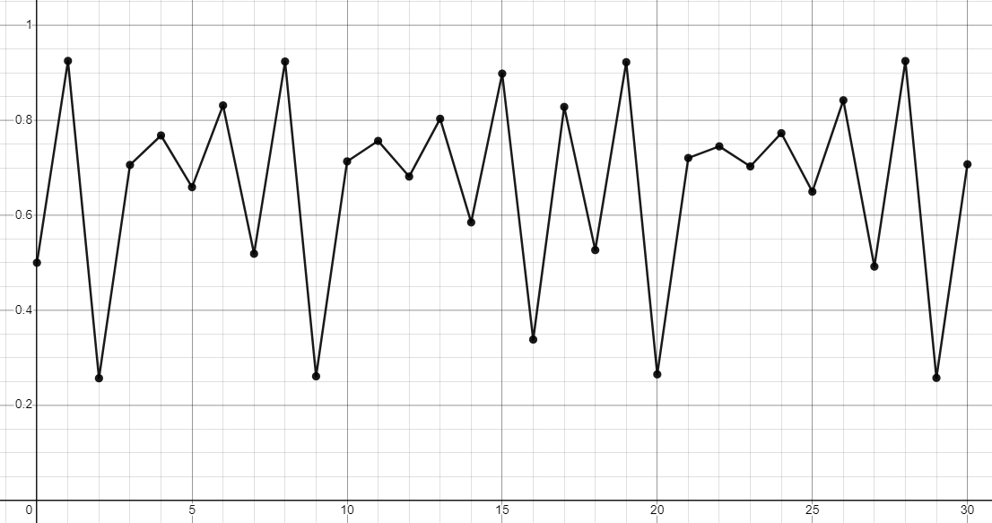
You can try the graph yourself here. Note the complex development and repetition. To properly illustrate the chaotic nature of this equation, a bifurcation diagram is used. On the diagram, the x-axis represents the value of the constant r and we plot on the y-axis all the values visited by xn after it settles into a cycle.
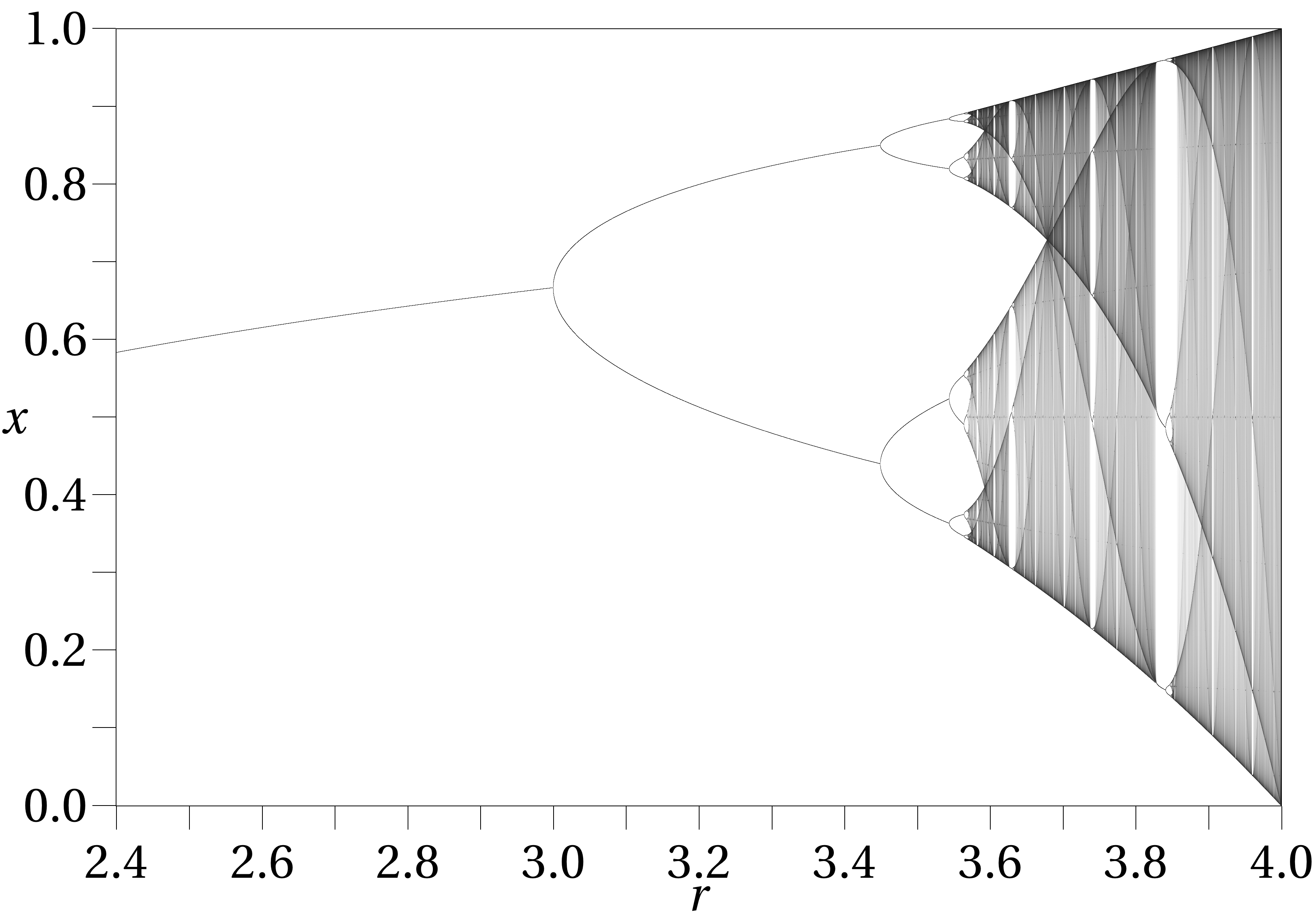
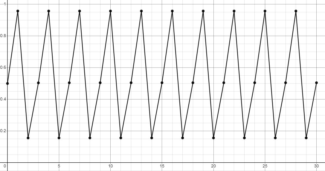
As you can see, until about r = 3, the iterative equation approaches a single value. For r = 2.5, that value is 0.6. From r = 3 to about r = 3.45, the equation approaches a cycle between two values. As r increases, the cycle rapidly increases in complexity until it becomes practically unintelligible. The previous graph, showing r = 3.7, is well within the chaotic region. There are brief interludes in this region, however. For example, below is the graph at r = 3.83.
The next step to this project is understanding the Mandelbrot set. The Mandelbrot set has been covered many times on this site, so I'll keep the definition brief. The Mandelbrot set is also defined as an iterative equation, this time it is xn+1 = xn2 + c. Many points, when iterated this way, fly off towards infinity. The remainder fall into cycles or fall towards a single point. These points which approach individual cycles or points can be graphed on a bifurcation diagram just like before. There is an important distinction, however. The Mandelbrot equation is typically iterated with 2-dimensional complex numbers, so our bifurcation diagram will be 3-dimensional.
The Code
In order to render this diagram, there are two steps that must be undertaken. First, the bifurcation diagram must be plotted. Second, it must be rendered. These two steps are encapsulated by the bifurcate and render programs, each of which come in a CPU variant and a GPU variant, the GPU versions being built with CUDA.
Plotting
The basic bifurcation algorithm works like this: iterate over all points in a range that includes the Mandelbrot set (I choose (-2, -1.5) to (1, 1.5), it helps that the range is square) and run the iterative equation. Each iteration produces a pair of floating-point values which we save, building a list of all the values visited as we iterate the equation. After each iteration, we scan the entire list to see if the current value is equivalent to any of the previous values, within some very small margin for error. This implies that we have reached a loop. We record the first value detected as part of the loop and all values visited after that as being the bifurcation sample. The collection of all samples forms something like a topographical map of the Mandelbrot set's bifurcation diagram.
There is another, more common approach generally used for bifurcation diagrams. Typically, you simply iterate the relevant equation many times and then record the next 100 or so values, under the assumption that by then it will have fallen into a cycle, and that that cycle will almost certainly be less than 100 values long. My algorithm's main advantage is storage space, which becomes a concern in this case. If you store 100 values, each composed of a 32-bit float, for each sample in a 4096 by 4096 grid, you'll be storing about 6.7GB of data! Seeing as how I like to use no fewer than 8192 by 8192 samples, this is an issue. Luckily, if we use loop detection to only save the values that we need, we end up using much less space. Remember: Large portions of the sample grid aren't even in the Mandelbrot set! So these samples will end up with a 4-byte value specifying the length of the loop as 0, rather than 400 bytes of 0s wasting space.
My algorithm is, on the other hand, slower. It requires performing a frankly unreasonable number of comparisons. A few things speed it up. First of all, the Mandelbrot set is symmetrical over the x-axis, so only compute one half of the set. Secondly, Don't start checking until you've done a lot of iterations. Thirdly, Don't check for loops longer than a few hundred iterations. Not checking for loops for a while also has another, very important improvement. Take a look at the path traced by the point (-0.6, 0.398), depicted as a black dot with a halo, when iterated seven times:
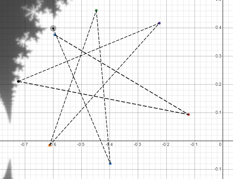
As you can see, the point nearly comes back to where it began. You might assume that this initial point falls into a cycle of length seven, but it is inside the main cardioid, and we happen to know categorically that all points inside the main cardioid approach a single value, effectively a cycle of length one. In fact, if you were to continue iterating this point, you'd see the path it follows would slowly spiral inwards toward the point (-0.45, 0.21). Unfortunately, our algorithm is not so clever. It will detect the cycle of 7 long before it detects the final location of the point, and although this has no effect on the final render (because by the time it detects the cycle, the different values are so close together that the distinction is irrelevant) this issue does result in many unnecessarily repeated values in the final binary, and results in many unnecessary comparisons during rendering. We solve this by ensuring we do two things: Firstly, we perform many iterations before we even start checking for loops. Contrary to what you might think, this actually speeds up the algorithm, because we skip over billions of comparisons, almost all of which turn out not to reveal any cycles. Secondly, we compare more recent iterations to our current value before the older ones, moving backwards to ensure we detect shorter loops before we detect longer ones.
Below I've included visualizations of the cycle data. The brightness of each pixel corresponds, non-linearly, to the length of the cycle found at that location. The left is generated with the naive cycle detection and the right with the improved cycle detection.
 |
 |
Cycle length as found by naive detection. 25.7 seconds to complete, 930KB of space used. |
Cycle length as found by improved detection. 0.62 seconds to complete, 651KB of space used. |
Even with the improvements, the GPU plotter, while fast, is severely limited by memory requirements in terms of what it can actually produce. The CPU plotter only needs to hold an individual sample in memory at a time, making it far more scalable. Unfortunately, the GPU plotter is only sufficient for producing test renders at this time. It is possible to remove this memory limitation by splitting the algorithm into many kernel calls. However, improvements to the CPU plotter proved sufficient for making high-quality renders for the time being. Should I ever choose to zoom in on the bifurcated Mandelbrot, I will absolutely begin by revisiting the GPU plotter.
Rendering
The rendering algorithm is quite a bit more sophisticated. It begins by sending rays in various directions, corresponding to individual pixels. In the original implementation, each ray would step inexorably forward at a very slow pace. As it passed through the sample space, its position would be converted to an index in the sample grid and used to detect whether the ray's height corresponds to any of the values visited by the sample at its position. If it does, the ray stops and the pixel corresponding to the ray is colored according to the ray's z-value. If the ray passes completely through the sample space, the pixel is colored black.
An improved version of the algorithm works by, first of all, advancing the ray forward to the sample space before beginning the iterations. Also, instead of stepping forward a set amount, it propagates according to an algorithm by Amanatides & Woo whereby the ray steps forward exactly as far as it needs to in order to get to the next sample that its path intersects.
The CPU version loads the data into a 3D jagged matrix for quick referencing. Unfortunately, this requires a pointer for every column in the sample grid as well as a pointer for each sample. With a 16,384 by 16,384 grid, accounting for the fact that only half of the grid is actually needed, this is 1.05GB on top of the 670MB that the actual data takes up. On the CPU this is acceptable, but not on the GPU. Some form of indexing is necessary, however, because the only alternative would be to have the threads iterate over the data to find their corresponding sample, which would be the dumbest possible way I could handle this situation. Instead, we pass the raw sample file to the GPU alongside an indexing table which provides the index, within the data, for every 16th sample. Each thread divides its ray's position by 16 and looks it up in the table to find the location of a nearby sample. It quickly iterates to the correct sample value and looks up the cycle data located there. The index table for a 16,384 by 16,384 sample grid takes up about 67MB.
Unlike the plotter, which is much better on the CPU at the moment, the renderer is and will always be many times faster on the GPU. It's job involves the transfer of much less data, as the sample grid is packed tightly by the plotting algorithm And doesn't need to be returned from the GPU. On an NVIDIA 3060, I have no issues loading a 20,480 by 20,480 sample grid (~1GB) onto the GPU alongside the blank image and lookup table. The amount of threads is typical for a kernel call and the amount of work done by each thread is substantial. The longest amount of time it has taken to render a frame is about 2 minutes, 20 seconds to render a 3840 by 2160 image of the plot, using a 20k sample grid.
The Final Render
And from the side... We see the bifurcation diagram of the logistic map! Well, more or less, it's upside down and stretched a bit but it's certainly there. In particular, if you trimmed everything off of the sides and just looked at the x-z plane, you'll see our original bifurcation diagram. If you can't quite see it, take a look at this gif on Wikipedia. This poses an interesting question. When we plot the bifurcation diagram of the Mandelbrot set, we see a resemblance to the logistic map's bifurcation diagram. So, if we plot the behavior of points on the logistic map the way we'd normally plot the Mandelbrot set, do we see a resemblance to the Mandelbrot set? We'll effectively be building a Mandelbrot renderer, but our inner loop will look like this:
	for (int i = 0; i < iter; i++) {
		sr = 1 - zr;

		zr_t = zr*cr*sr + zr*ci*zi + zi*zi*cr - zi*ci*sr;
		zi = zr*ci*sr + zi*cr*sr + zi*zi*ci - zr*cr*zi;
		zr = zr_t;

		double sqr_abs = zr*zr + zi*zi;
		if (sqr_abs > 2000) {
			img[y*width + x] = (uint8_t) (i % 255);
			break;
		}
	}
The modified iteration formula is the complex expansion of the logistic map formula Zn+1 = C · Zn(1 - Zn). Note that the letters have been changed to match the Mandelbrot formula. We also start with Z0 = 0.5 + 0i instead of 0 + 0i, which is typical with the logistic map.
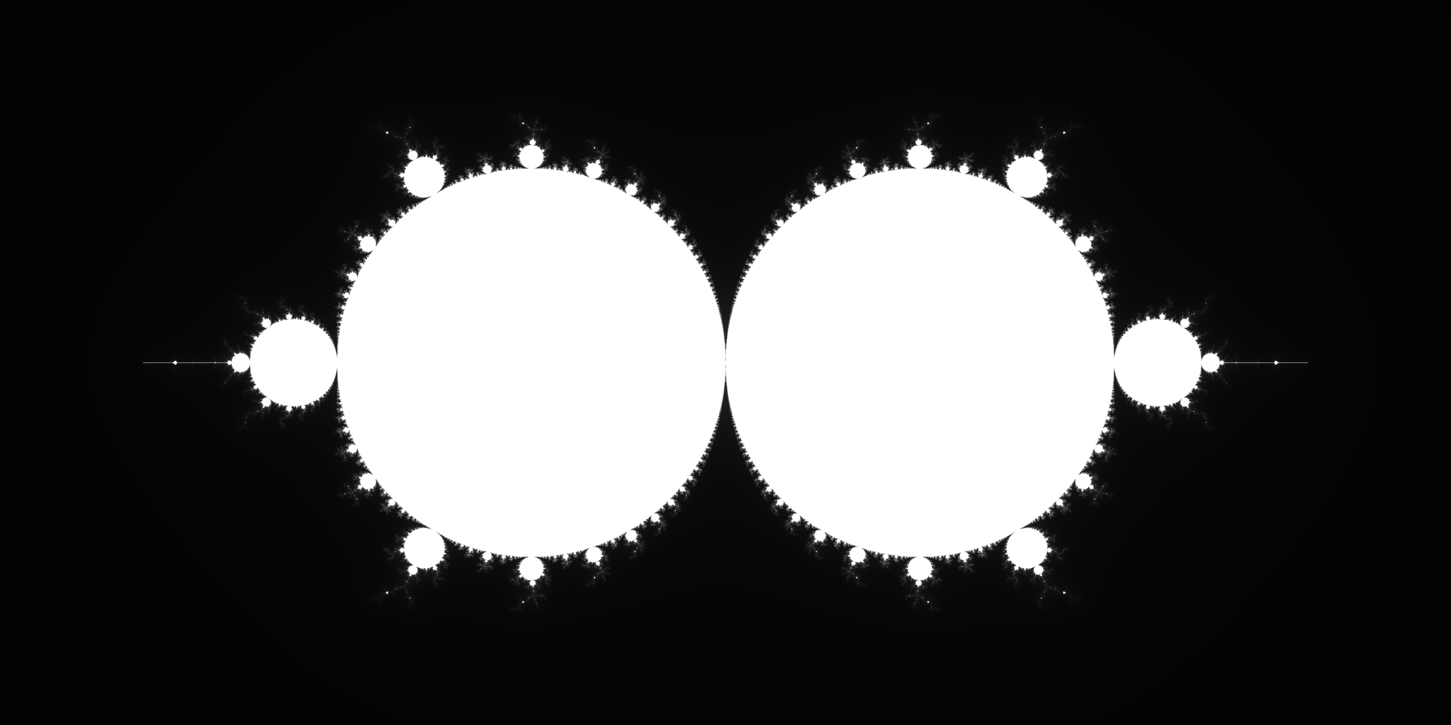
We certainly do see a resemblance! This equation is its own interesting fractal and it contains many of the patterns found in the Mandelbrot set. If, however, you were hoping for a stronger resemblance, then you're in luck:
Much like the Mandelbrot set itself, this fractal contains an infinite number of mini-Mandelbrots!
Errors
Included below are some test renders that didn't come out quite right...


Frame writing errors.
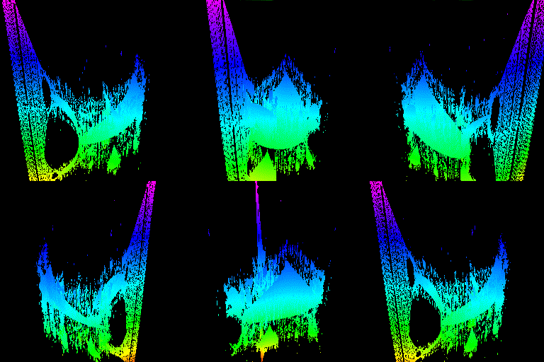
An error converting rays from world space to sample space effectively caused the rays to be refracted when they approached the Mandelbrot set.
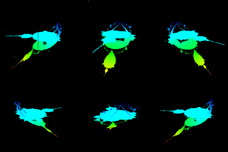
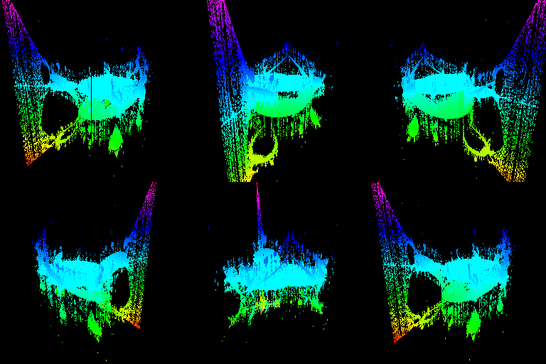
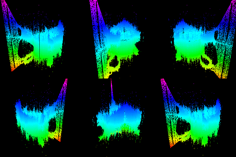

A variety of cycle detection and recording errors.


Samples that were encoded row-first were being read column-first. On the left-most render, the raycasts also bailed way too early.
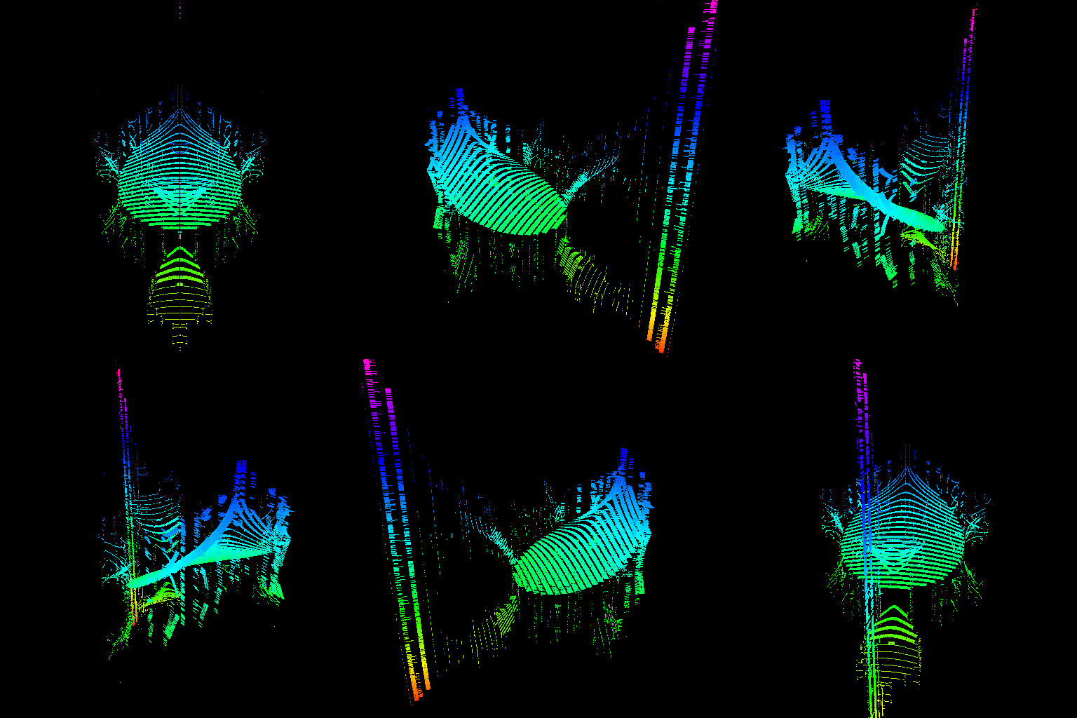
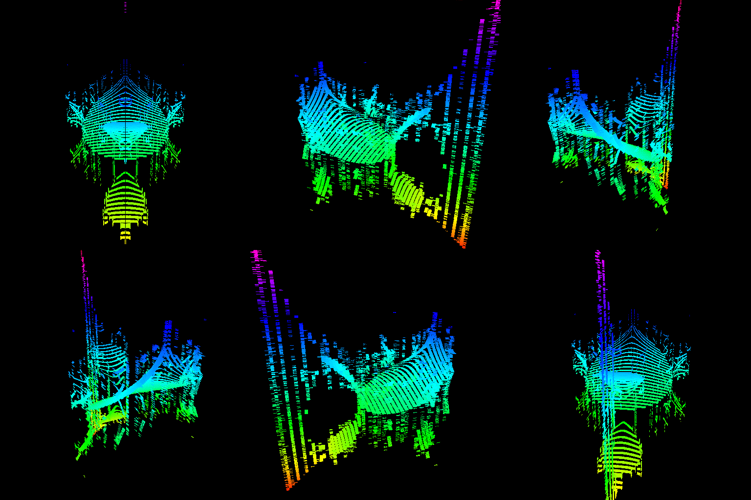
GPU threads were not properly seeking to their sample value. The render on the right was actually made by intentionally disabling the seeking code, proving that it was the cause of the issue.

Frame writing errors on the logistic map fractal zoom.
Encountered the floating-point precision barrier while rendering the logistic map fractal.